This week in Pre-Calculus 11 we expanded our knowledge on trigonometry. We started off by reviewing Math 10 trig, then moved into unit circles and special triangles. We learned how to do trig without calculators by using special triangles. We reformed SOH CAH TOA to be able to apply it in non-right triangles. Another thing we learned was Sine and Cosine Law.
Category Archives: Math 11
Week 14 – Multiplying and Dividing Rational Expressions
This week in Pre-Calculus 11 we started the Radical Expressions and Equations unit. In lesson 7.2 we review multiplying and dividing fractions then learned how to divide and multiply rational expressions.
Example 1:
Before simplifying state the restrictions. Restrictions always come from the denominator.
z 0 and y
0
Simplify
Stop when you can’t simplify any further.
When multiplying or dividing single variable expressions you need to factor. Factor before stating restrictions because when you factor you can extend trinomials so you have more zeroes. Once the restrictions are stated then you simplify.
How to multiply or divide single variable expressions:
1. Factor
2. State Restrictions
3.Simplify
Week 12 – Absolute Value Functions
This week in Pre-Calculus 11 we started a new unit. This unit includes absolute values and how we can graph them. I will show you how to graph an abosolute value linear function. There are steps that we need to follow when dissecting an equation.
1. Graph the parent function
2. Find the y-intercept
3. Find the slope
4. Graph absolute value
5. Find the critical point (solution)
Something to look for when graphing linear absolute value functions is the x-intercept. This is important because the x-intercept is the critical point, the point where the graph changes direction. Some equations will have no solution which means they don’t touch the x-axis.
Week 13 – How to graph reciprocal functions
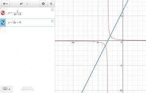
This week in Pre-Calculus 11 we learned about reciprocal linear and quadratic functions. We learned how to solve the functions algebraically and graphically. My preferred method is graphing to solve because it is a visual for me to see even though it is specific it helps work it out.
How to graph a reciprocal linear function:
1. Graph line (parent function)
2. Plot invariant points (y=1 or y=-1)
3. Asymptotes —> x-intercepts = vertical asymptotes
—> y=0 which is the horizontal asymptotes
How to graph a reciprocal quadratic function:
1. Graph parabola (parent function)
2. Invariant points (y=1 or y=-1)
3.Asymptotes —> x-intercepts = vertical (2 possible solutions)
—> y=0 which is the horizontal asymptote
Week 11 – Graphing Linear Inequalities in Two Variables
This week in Pre-Calculus 11 we reviewed linear graphing (y=mx+b) from Math 10 and expanded on it. So instead of looking for just one answer of y we look for the possibilities of y. Also we use inequalities instead of an equal sign. I will be blogging about Graphing linear inequalities in two variables (x and y). Solutions to linear inequalities in two variables is represented by the boundary lines and shading on one side.
The inequality used decides what the boundary line looks like.
A solid line is greater/less than or equal to…
A broken line is greater/less than…
When you shade you need to test one of point on either side of the line. If the answer is true such as (y<x+2 —> 0<0+2 —> 0<2) then shade on that side of the line. In the example I used (0,0) as my test point. If it isn’t true choose a point on the other side of the line and test that. Try and use (0,0) as your test point it makes it easier and leaves less room for mistakes.
Examples
This when y is greater than x+2. So the line is broken and the shading is above.
In this graph y is less than x+2. So the line is broken and the shading is on the bottom.
This graph is saying y is greater than or equal to x+2. So the boundary line is solid and the shading is above.
y is less than or equal to x+2 in this graph. So the boundary line is solid and the shading is below.
Week 10 – Discriminant
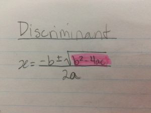
This week in Pre-Calculus 11 we reviewed for our midterm. So we are suppose to blog about something we haven’t blogged about yet. I chose the discriminant because it was something I struggled with until review this week. The discriminant is how we determine how many solutions there are. Here is how to find the discriminants . This connects to the quadratic formula, the pink is the discriminant formula.
So you can have 2 solutions, 1 solution, or no solution.
a=1, b=-6, c=5
Plug in a, b, and c.
36-20
16 gives 2 solutions
This parabola crosses the x-axis twice giving us two solutions.
a=1, b=-6, c=9
Plug in a, b, and c.
36-36
0 gives one solution
The parabola crosses the x-axis once meaning there is only one solution.
a=1, b=-6, c=13
Plug in a, b, and c.
36-52
-16 gives no solution
The parabola never crosses the x-axis so there is no solution.
Week 9 – Equivalent Forms of the Quadratic Functions
This week in Pre-Calculus 11 we learned about equivalent forms of the quadratic functions, analyzing , and applying what we learned this unit into word problems. This post I am going to focus in on equivalent forms of the quadratic functions. There are three equivalent forms of the quadratic function the general, standard, and factored form. We are going to look on the general and standard form.
General form —>
Standard form —>
When changing between general and standard form you have to use the completing the square method to do so.
Week 8 – Translation and Scale
This week in Pre-Calculus 11 we learned about quadratic functions. We learned about the properties, looking at an equation and extracting information for the parabola, and analyzing $latexy=a(x-p)^2+q$. I am going to focus on looking at an equation and extracting information for the parabola. Translations can go up and down or side to side. Scales can either stretch or compress the parabola.
$latexy=x^2+p$ —> The parabola moves up/down because there are no brackets around $latexy=x^2+p$
$latexy=(x-p)^2$ —> The parabola moves left or right because there are brackets around x-p. When p is negative the parabola moves to the right but if p is positive the parabola moves to the left.
$larexy=ax^2$ —> The parabola stretches when a is greater than 1. If a is less than one the parabola compresses. Also if a is negative the parabola will open down instead of up.
Week 6 – Perfect Square Trinomials
This week in Pre-Calculus 11 we learned about perfect square trinomials. We learned how to regonize and factor them. How can you identify perfect square trinomials? You need to look at each term.
The first term is a perfect square
The third term is a perfect square that must be positive.
The second term can be positive or negative.
Week 5 – Ugly fractions
This week in Pre-Calculus 11 we learned about factoring polynomials. Ms. Burton gave a very useful acronym Can Divers Pee Easily Underwater.
Common
Difference of squares
Pattern
Easy
Ugly
These are the steps that help break down a polynomial and properly factor it. In this blog post I am going to focus on Ugly polynomials because it was something I struggled with. There are multiply ways to factor ugly polynomials but I prefer the square method. This is my favourite because it looks nice, its easy to understand, and breaks it down right to the answer.
First I identified is there was anything in common, if there was a difference of squares, or a pattern.
I noticed the pattern of a normal polynomial, then asked if it is easy or ugly? You can identify this by looking infront of the squares variable, so if there is no coefficient then it is easy but if there is a coefficient then it is ugly. So this polynomial is ugly.


