
This week in Pre-Calculus 11 we reviewed linear graphing (y=mx+b) from Math 10 and expanded on it. So instead of looking for just one answer of y we look for the possibilities of y. Also we use inequalities instead of an equal sign. I will be blogging about Graphing linear inequalities in two variables (x and y). Solutions to linear inequalities in two variables is represented by the boundary lines and shading on one side.
The inequality used decides what the boundary line looks like.
A solid line is greater/less than or equal to…
A broken line is greater/less than…
When you shade you need to test one of point on either side of the line. If the answer is true such as (y<x+2 —> 0<0+2 —> 0<2) then shade on that side of the line. In the example I used (0,0) as my test point. If it isn’t true choose a point on the other side of the line and test that. Try and use (0,0) as your test point it makes it easier and leaves less room for mistakes.
Examples
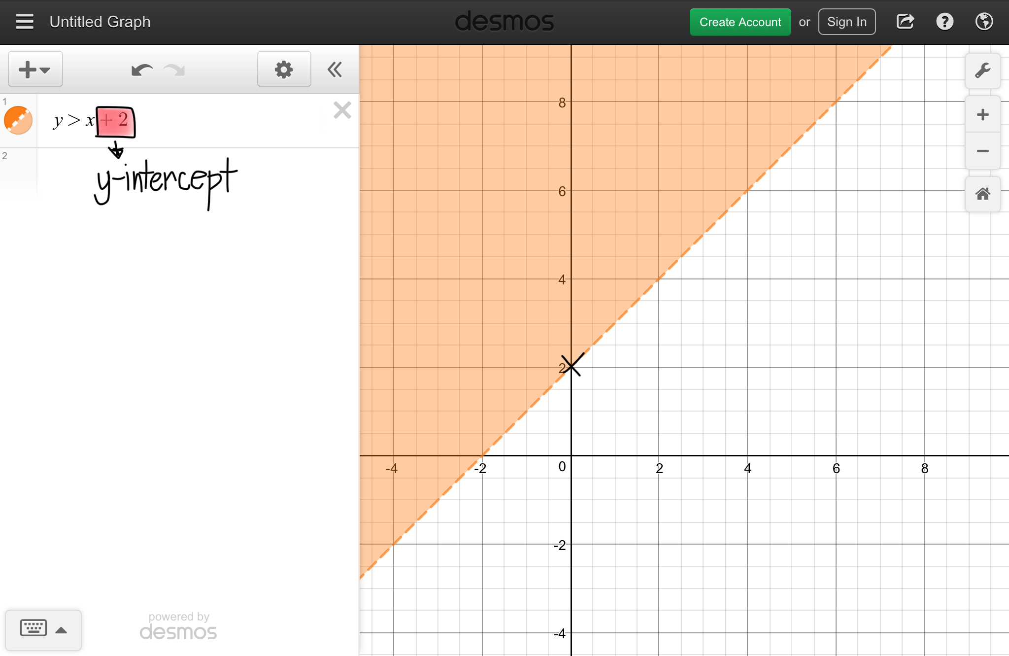
This when y is greater than x+2. So the line is broken and the shading is above.
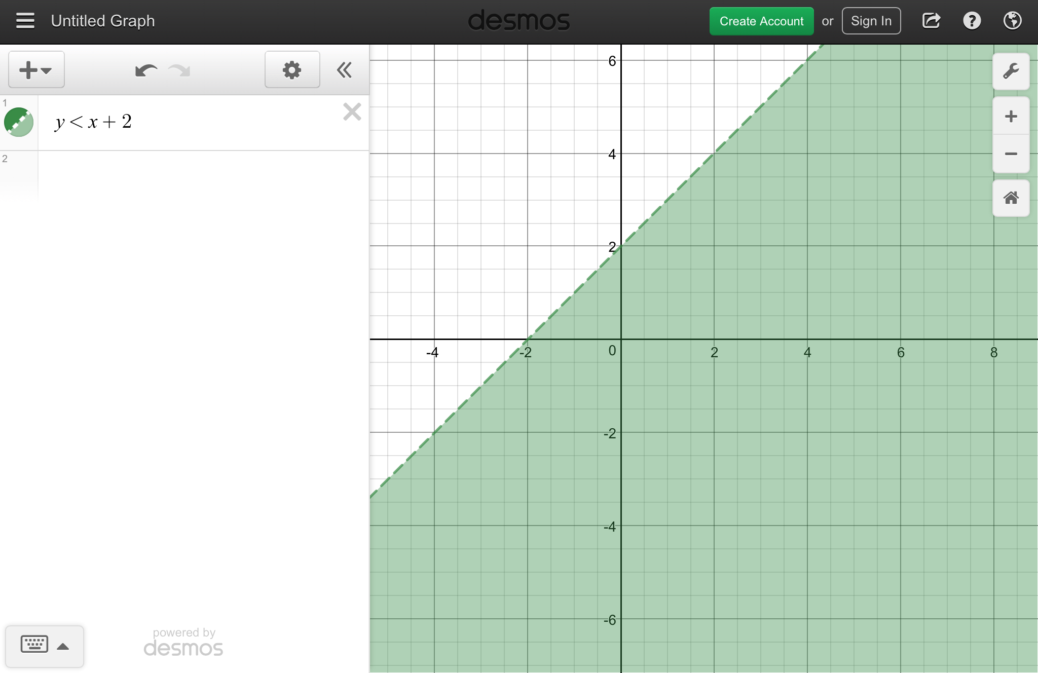
In this graph y is less than x+2. So the line is broken and the shading is on the bottom.

This graph is saying y is greater than or equal to x+2. So the boundary line is solid and the shading is above.

y is less than or equal to x+2 in this graph. So the boundary line is solid and the shading is below.