Week 18 – My TOP 5 things from PC 11

  1. Quadratic Inequalitys: I chose this subject because it was a harder one to grasp and understand so i had to look at it differently and access online materials which changed how i look at learning new things
  2. Rational Expressions and equations: I chose this subject because it was when i noticed how bad my attention to detail was and forced me to check my work more thoroughly.
  3. Quadratic formula: I choose this subject because  it was when i started to see how physic connect to math  with formulas.
  4. Quadratic Parabola: I choose this subject because it was interasting to have to visually identify  diagrams extstensively which i am not used as i learn by applying logic to problems
  5. Factoring: I chose this subject because it was when i learned how much farther and more steps are required in more advanced math in precalc 11 with simplifying after having two different factors

Week 17 in Precalc 11 – Sine and Cosine law


This week in math we learned how to use the Sine and Cosine law. I choose this skill because it was an improved version of past formulas that used trignometric ratios and inverse trigonmetric ratios and could apply to all triangles. This is an important skill to finding the length and angles of any triangle in order to solve it not just right angle ones.

Sine Law (Law of Sines)

The Law of Sines states that in any triangle equation, the ratio of the length of a side to the sine of its opposite angle is constant. This can be written as:

equation

Steps to Use the Sine Law:

1. Identify the known values in the triangle (sides and angles).
2. Set up the ratio according to the Sine Law.
3. Solve for the unknown value.

Example:

Given triangle equation, where:
equation
equation
equation

Find side equation.

Solution:

1. Identify the known values:
equation
equation
equation

2. Set up the ratio:
equation

3. Plug in the known values:
equation

4. Solve for \( b \):
equation
equation
equation
equation

Cosine Law (Law of Cosines)

The Law of Cosines relates the lengths of the sides of a triangle to the cosine of one of its angles. It can be written as:

equation

Steps to Use the Cosine Law:

1. Identify the known values in the triangle (sides and angles).
2. Set up the equation according to the Cosine Law.
3. Solve for the unknown value.

Example:

Given triangle ( ABC ), where:
equation
equation
equation

Find side c.

Solution:

1. Identify the known values:
equation
equation
equation

2. Set up the equation:
equation

3. Plug in the known values:
equation
equation
equation
equation
equation
equation

These examples demonstrate how to apply the Sine and Cosine Laws to find unknown sides or angles in a triangle.

Week 16 in Precalc 11 – Finding Trigonometric Ratios

This week in math we learned how to find exact trigonometric ratios when given an exact point on the terminal arm or a single trignometric ratio. This skills is important cause it is great for encreasing spatial awerness and can be applied to other subjects like physics. I choose this subject because of how little information is needed to find a ton of values.

1. Finding the Exact Trigonometric Ratios for Rotation Angles from 0° to 360° Given a Point on the Terminal Arm

Steps:

1. Identify the Coordinates: Determine the coordinates (x, y) of the point on the terminal arm.

2. Calculate the Radius (r): Use the formula equation to find the radius (hypotenuse).

3. Find the Trigonometric Ratios:
– Sine (sin θ): equation
– Cosine (cos θ): equation
– Tangent (tan θ): equation

Example:

Given the point (3, 4) on the terminal arm:
equation
equation
equation

Trigonometric Ratios:
equation
equation
equation

2. Determining Trigonometric Ratios for a Rotation Angle from 0° to 360° Given a Different Trigonometric Ratio for the Angle

Steps:

1. Identify the Given Ratio: Determine which trigonometric ratio is provided (e.g., sin, cos, tan).

2.Determine the Quadrants: Based on the given ratio’s sign, determine the possible quadrants where the angle could lie.
– Sine (sin θ):
– Positive in Quadrants I and II
– Negative in Quadrants III and IV
– Cosine (cos θ):
– Positive in Quadrants I and IV
– Negative in Quadrants II and III
– Tangent (tan θ):
– Positive in Quadrants I and III
– Negative in Quadrants II and IV

3. Use Reference Angles: Find the reference angle (θ) using the inverse function of the given ratio.

4. Determine the Actual Angles: Add or subtract the reference angle from 180° or 360° based on the quadrants identified.

Example:

Given equation:

– Since equation is positive, θ could be in Quadrant I or II.
– Reference angle equation.

Actual angles:
– In Quadrant I: equation
– In Quadrant II: equation

To find other trigonometric ratios at these angles:
– For equation:
equation
equation
equation

– For equation
equation

equation
equation

Using these steps and examples, you can determine the exact trigonometric ratios for any given point or provided ratio.

Week 15 in Precalc 11 – Rotation Angle and Refrence Angle

This week in Precalc I choose the rotation angle and refrence angle because the refrence angle was new to me and looked like an angle I had never thought of in math 10. These angles are important because they make it possible to evaluate trigonometric functions for angles outside the first quadrant. They can also be used to find (x,y)coordinates for those angles.

Steps to Find the Rotation Angle
1. Determine the Quadrant:
– Identify which quadrant the angle lies in based on its degree measure.
– Quadrant I: equation to equation
– Quadrant II: equation to equation
– Quadrant III: equation to equation
– Quadrant IV: equation to equation

2. Calculate the Rotation Angle:
– If the angle is between equation and equation, it is already a rotation angle.
– If the angle is greater than equation or less than equation, subtract or add equation repeatedly until the angle falls between \(0^\circ\) and \(360^\circ\).

Steps to Find the Reference Angle
1. Identify the Quadrant:
– Use the same quadrant identification as above.

2. Calculate the Reference Angle:
– Quadrant I: The reference angle is the same as the given angle.
equation
– Quadrant II: Subtract the angle from equation.
equation
– Quadrant III: Subtract equation from the angle.
equation
– **Quadrant IV**: Subtract the angle from equation.
equation

### Example
Let’s find the rotation and reference angles for equation.

Rotation Angle
1. **Determine the Rotation Angle*:
equation is greater than equation. Subtract equation to bring it within the range.
equation
– The rotation angle is equation.

Reference Angle
1. Identify the Quadrant:
equation lies on the boundary between Quadrant I and Quadrant II, but it is typically considered to be in Quadrant I.

2. Calculate the Reference Angle:
– Since equation is in Quadrant I, the reference angle is the same as the given angle.
equation

So, for equation, the rotation angle is \(90^\circ\) and the reference angle is equation.’

Reference Angle Calculator | Pi Day

link

Week 14 in Precalc 11 – Solving Rational Equations

This in Precalc we learned how to solve rational equation  I choose this subject because it was an interesting application of simplyfiying rational expressions using addition , subtractions, multiplication and division. Solving rational equations is important because they are a useful tools for representing real-life situations and for finding answers to real problems and finding unkowns.

Steps to Solve Rational Equations (note: this is one method to solve Rational Equations using the LCD )

1.Identify the Denominators: Identify all the denominators in the equation if needed find the value for x on the deminator that would make the denomiator equal 0 that is your non-permissable value.

2. Find the Least Common Denominator (LCD): Determine the least common denominator of all the rational expressions in the equation.

3. Clear the Denominators: Multiply both sides of the equation by the LCD to eliminate the denominators. This step turns the rational equation into a polynomial equation.

4. Simplify the Equation: Distribute and combine like terms to simplify the equation.

5. Solve the Resulting Equation: Solve the simplified polynomial equation using appropriate methods (factoring, quadratic formula, etc.).

6. Check for Extraneous Solutions: Substitute the solutions back into the original rational equation to ensure they do not make any denominator zero. Discard any solutions that do.

Example:

Solve the rational equation: equation.

Step 1: Identify the Denominators
The denominators are equation and equation so are non permissible values for x are -1, 2.

Step 2: Find the Least Common Denominator (LCD)
The LCD of equation and equation is equation.

Step 3: Clear the Denominators
Multiply both sides of the equation by the LCD equation:

equation

Distribute the LCD to each term:

equation

Step 4: Simplify the Equation
Distribute and combine like terms:

equation

Combine like terms on the left side:

equation

Move all terms to one side to set the equation to zero:

equation

Step 5: Solve the Resulting Equation
This is a quadratic equation, so we can solve it using the quadratic formula \equation, where equation, equation, and equation:

equation
equation
equation
equation
equation

The solutions are equation and equation.

Step 6: Check for Extraneous Solutions
Substitute equation and equation back into the original equation to ensure they do not make any denominator zero. Since neither value makes equation or equation equal to zero, both are valid solutions.

Final Answer

The solutions to the rational equation equationare equation and equation.

Week 13 in Precalc 11 – Adding and Subtracting Rational Expressions

This week in Precalc we learned how to simplify add, and subtract rational expression I choose this subject because i was intriged about cancling out factor in the numerator and denominator and it was very hard for me to understand at first. Learning how to properly add and subtract rational expressions can save you time simplify and allows you to simplify more advanced expressions that have variables and polynomials

To add and subtract complex rational expressions, follow these steps:

1. Find a common denominator: Identify the least common denominator (LCD) for the rational expressions involved. This is the least common multiple of the denominators.

2. Convert each fraction: Rewrite each fraction so that its denominator matches the common denominator found in step 1.

3. Perform the operation: Add or subtract the numerators of the fractions while keeping the common denominator unchanged.

4. Simplify if necessary: Simplify the resulting fraction by factoring and canceling out common factors.

Here’s an example:

Let’s add the following two complex rational expressions:

equation

1. Find the least common denominator (LCD), which is equation.
2. Convert each fraction:
equation
equation
3. Add the converted fractions:
equation

4. The result can be further simplified if possible.

How to simplify a rational expresion with common factors in the numerator and denominator:

Adding and Subtracting Rational Expressions

Week 12 in Precalc 11 – Quadratic and Linear inequalities

This week we learned how to solve and graph inequalites. I choose this subject because it was an interesting application of algebra and solving with quadratic equations

I learned how to solve and graph linear inequalities
1. * Start by identifying the linear inequality in the form equation, equation, equation, or equation, where equation, equation, and equation are constants.
2.  Solve the inequality for \(x  just like you would solve an equation, using inverse operations. Remember to reverse the inequality sign if you multiply or divide by a negative number.
3. Represent the solution on a number line. Use an open circle for equation or equation inequalities and a filled circle for equation or \( \leq \) inequalities. Shade the region to the right for equation or equation inequalities and to the left forequation or equation inequalities.

Example:
Let’s solve and graph the inequality equation.
1. Identify the inequality: equation.
2. Solve for equation: Subtract 3 from both sides to get equation, then divide by 2 to get equation.
3. Graph the solution: On a number line, put an open circle at 2 and shade to the left.

**Quadratic Inequalities:**
1. Identify the quadratic inequality in the form equation, equation, equation, or equation, where equation, equation, and equationare constants.
2.  If possible, factor the quadratic expression to find its roots. If factoring is not possible, use the quadratic formula to find the roots.
3.  Use the roots to determine the intervals where the inequality is true based on the signs of the quadratic expression within those intervals.
4.  Represent the solution on a number line, using open or filled circles depending on whether the inequality is strict or non-strict, and shade the appropriate intervals.

Example:
Let’s solve and graph the inequality equation.
1. Identify the inequality: equation.
2. Factor the quadratic:equation, so the roots are equation and equation.
3. Determine intervals: The intervals to consider are equation, equation, and equation. Test a value from each interval to determine the sign of the expression in that interval (e.g., equation) gives a positive value, equation gives a negative value, and equation gives a positive value).
4. Graph the solution: On a number line, use open circles at 1 and 3 and shade the intervals where the inequality is true (to the left of 1 and to the right of 3).

These steps should help you solve and graph both linear and quadratic inequalities effectively.

Here are the steps to graph quadratic inequalities

Quadratic Inequalities - GCSE Maths - Steps, Examples & Worksheet

Week 11 in Precalc 11 – Quadratic Functions Applications

This week we learned applications of quadratic functions with word problems. I choose this subject because I was interested in how these quadratic lines could be applied to real life situations. Quadratic applications are important because they allow you to   learn about different ways to see math problems and numbers in general with variables.

1. Understand the Problem: Read the word problem carefully to identify what information is given and what needs to be found. Look for keywords that indicate a quadratic relationship, such as “area,” “height,” “distance,” “time,” etc.

2. Define Variables: Assign variables to the quantities mentioned in the problem. For example, if the problem talks about the area of a rectangular garden, you can let  x  represent the length and  y  represent the width unless given.

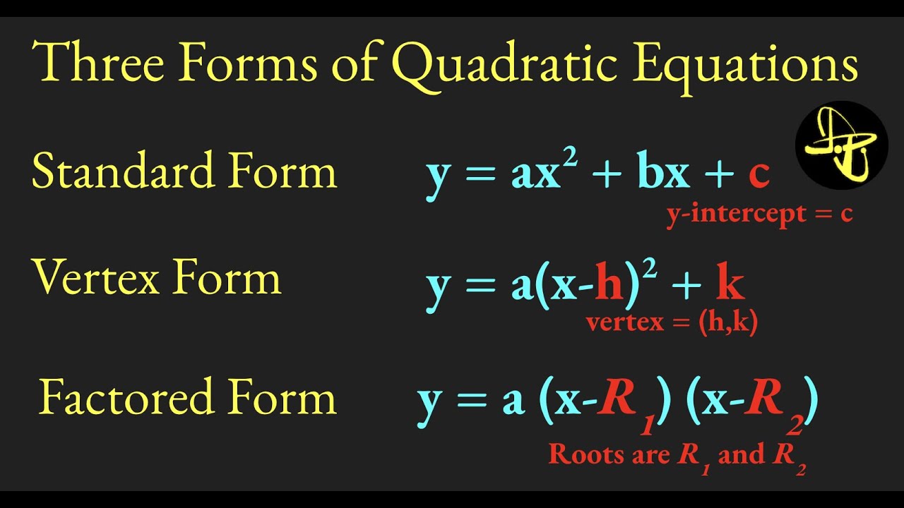
3. Turn it into a Quadratic Equation: Use the given information to formulate a quadratic equation that represents the problem. This equation will typically have the form  y = ax^2 + bx + c , where a , b , and  c  are constants.

4. Solve the Equation: Depending on the problem, you may need to solve the quadratic equation to find the values of the variables. You can use factoring, the quadratic formula, or completing the square to solve for  x  or  y .

5. Interpret the Solution: Once you have the solution, interpret it in the context of the problem. Sometimes, you may need to discard extraneous solutions that don’t make sense in the given situation.

Here’s an example to illustrate these steps:

Example Problem:A ball is thrown upward from the top of a 30-meter building with an initial velocity of 20 m/s. The height of the ball above the ground at time \( t \) seconds is given by the equation equation. When does the ball hit the ground?

Steps to Solve:

1. Understand the Problem: We need to find the time at which the ball hits the ground, which corresponds to when the height \( h(t) \) is 0.

2. Define Variables: Let t represent time in seconds.

3. Formulate the Quadratic Equation: The equation for the height of the ball is given as equation. Set \ h(t)  to 0 and solve for  t :
equation

4.Solve the Equation: Use the quadratic formula equation with equation, equation, and equation to find the values of equation:
equation
equation
equation
equation
equation

5. Interpret the Solution: Since time cannot be negative in this context, we discard the negative solution. The ball hits the ground after approximately equation seconds.

This process demonstrates how quadratic functions can be applied to real-world scenarios to solve problems related to motion, distance, height, and other physical quantities.

Week 10 in Precalc 11 – Different Quadratic Forms

I choose what we learned about going from general to standard form quadratic functions and how the different forms can be used to graph the function. I choose this topic because it allows you to graph and figure out the different parts of a quadratic function with different form of the function instead always converting it to vertex form and we also learned about converting general to standard form which is nessacary when using standard form quadratic functions. We learned that the factored form helps in quickly identifying the roots (zeros) of the quadratic equation, which are where the function intersects the x-axis. It’s useful for solving quadratic equations and getting the vertex by adding the two roots and diving by two to find the x cordinate of vertex which can be put in the equation to find the y-cordinate. the general form provides a comprehensive view of the quadratic equation, showing the coefficients of x², x, and the constant. It’s often used in algebraic manipulations, such as completing the square to find the vertex form or solving systems of quadratic equations. the Standard form highlights the vertex of the quadratic function, which is the highest or lowest point on its graph depending on the quality of the coefficient. It’s crucial for graphing quadratic functions accurately and understanding transformations like shifts, stretches, and compressions. This is also how you convert standard for to general form

Three Forms of Quadratic Equations - YouTube

Converting from Standard Form to General Form (With Coefficient on equation)
Starting with the standard form equation:

1. Start with the Standard Form: equation
2. Expand the Equation: equation
3. Group the Terms: Group the quadratic term equation and the linear term equation together: equation
4. Factor Out the Common Factor equation
5. Complete the Square: Add and subtract equation inside the parentheses: equation
6. Factor and Simplify:equation
7. Distribute \a  and Simplify Further: equation
8. Combine the Constants: equation
9. General Form: equation

Converting from Standard Form to General Form (Without Coefficient on \( x^2 \))
Starting with the standard form equation

1. Start with the Standard Form: equation
2. Complete the Square: Add and subtract equation inside the parentheses: equation
3. Factor and Simplify: equation
4. General Form: equation

In both cases, you end up with the quadratic function in general form, which is equation, where equationand equation when there is a coefficient on the equation term, and equation and equation when there is no coefficient on the equation term.

Let’s work through an example of converting a quadratic function from standard form to general form step by step.

Example:
Convert the quadratic function equation from standard form to general form.

Steps to Convert from Standard Form to General Form:
1. Start with the Standard Form: equation
2. Factor Out the Coefficient equation: Since equation, we factor outequation
3. **Complete the Square Inside the Parentheses:**
– Add and subtract equation inside the parentheses: equation
– Rewrite the equation: equation
4. Distribute 2 and Simplify: equation
5. **Combine Constants:** equation

Now, the quadratic function is in general form: equation. In this form, equation and equation, which represent the vertex of the parabola.

So, the quadratic function equation in standard form is equivalent to equation in general form.

Three Forms of Quadratic Equations - YouTubelink

Week 9 in Precalc 11 – Quadratic Functions

I choose Quadratic Functions because they were an interesting advanced version of normal function and graphs. Analyzing Quadratic function is important in order to understand its components and predict the trends of its graphed form. These are the steps in order to fully analyze a quadratic function.

1. First we must understand what a quadratic function is when in the form equation where a, b , and  c  are constants. The graph of a quadratic function is a parabola.

2. Identify the Key Features:
– Vertex: The vertex of a parabola is the highest or lowest point on the graph and can be found with -b being the x cordinate and c being the y .
– Axis of Symmetry: The axis of symmetry is the vertical line that passes through the vertex. It is given by finding the x cordinate of the vertex.

–  Slope: The a is how wider the parobola is with higher the number the thiner paraobola
– Intercepts The x-intercepts are the points where the graph crosses the x-axis, and the y-intercept is the point where the graph crosses the y-axis. To find the x-intercepts, set equation and solve for x . The y-intercept is equation.

3. Determine the Direction of Opening:
– If a > 0 , the parabola opens upward.
– If a < 0 , the parabola opens downward.

4. Plot Points and Sketch the Graph:
– Use the vertex, intercepts, and symmetry to plot points and sketch the graph of the quadratic function.

5. Analyze the Graph:
– Determine the domain and range of the function.
– Identify any maximum or minimum values.
– Check for symmetry and whether the function is increasing or decreasing.

Sure, let’s analyze the quadratic function equation using the steps we discussed earlier:

1. Understand the Function: The given quadratic function is in the form equation.

2. Identify Key Features:
– Vertex: The vertex form of a quadratic function is equation, where (h, k) is the vertex. In this case, the vertex is (-5, 4).
– Axis of Symmetry: The axis of symmetry is given by the equation \x = -5 .
– Intercepts: To find the x-intercepts, setequation. However, this function has no real roots because the square term is always non-negative. The y-intercept is equation.

3. Direction of Opening: Since the coefficient of the squared term is positive, the parabola opens upward.

4. Plot Points and Sketch the Graph:
– Plot the vertex (-5, 4) and the y-intercept (0, 29). Since there are no real x-intercepts, the graph does not intersect the x-axis.
– Use the symmetry to plot other points if needed.

5. Analysis:
– Domain: All real numbers.
– Range: equation (since it opens upward).
– Minimum: The vertex (-5, 4) is the minimum point.
– Increasing or Decreasing: The function increases as you move to the right from the vertex and decreases as you move to the left.