Solving Quadratic Systems of Equations Algebraically

This week in math I learned how to solve a quadratic system of equations algebraically.

First, we need to know that a quadratic system is similar to a linear system but what makes it different is that it has a degree of two.  Although similarly our end goal is to find the coordinates of the points where each equation intersect with each other.

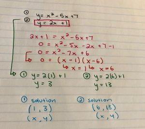
If my two quadratic equations were:

First I want to get either X or Y by itself.  To do this I must rearrange one of the equations.  In this case, both are already arranged.  I will use the second one because I find it easier to use due to the fact it does not have a square root.

Now that I have Y and is equal to 2x + 1 I will take 2x + 1 and input it into the first equation wherever Y is.

Now I have a quadratic equation that I need to factor.

After factoring I have my X intercepts which are equal to 1 and 6.  To find my values of Y I will take each X intercept and use the first equation and replace X  with my intercepts 1 and 6 to determine it’s Y partner.

Now you have the partners.

Finally you have your two solutions of coordinates of where the quadratic system intersects.

Math Review

This week in math I reviewed how to simplify an entire radical into a mixed radical.

First we need to know the difference between a mixed and an entire radical.  An entire radical only has a radicand and a mixed radical has a radicand and a coefficient.  As seen below:

To change an entire radical into a mixed one we need to know how to factor.  When factor we take out all the multiples of 2 and once you exterminate multiples of 2 than you move onto three and so on. Here are two examples below:

Finally, if it is a square root you are looking for the pairs that make perfect squares and bringing them outside of the radicand as the coefficient. The number or numbers left over become the radicand.  If there is more than one number left over you simply multiple them together to create that radicand.

Now you have a mixed radical.

Standard Form of a Parabola Equation

This week in math we learned about the standard form of a parabola equation.

When using the standard form of the equation it is very useful because it reveals a lot about how to graph the equation without a table of values.

First of all, standard equation is: y = a+ q

At first glance, it looks very confusing but with the information we have you are able to found out the directions opening, vertex, axis of symmetry, intercepts, domain, and range.  Some information is found easily by just looking at the values that correspond with the variables but in some cases, the information you will have to be pieced together.

When looking at y = a+ q the different variables tell us multiple things:

A, whether the parabola opens up or down and if the vertex is a maximum or minimum vertex.  If the value of a is negative than the parabola opens down and we know the vertex will be at its maximum.  If the value is positive then we know the parabola opens up and the vertex will be at its minimum.

P, tells you the horizontal translation.  Also known as to when starting at 0 on the x-axis if you will be sliding left or right.  Another thing to note is if the p-value follows a positive you will be sliding to the left (negative) by that many intervals and if the p-value follows a negative you will be sliding to the right (positive) by that many intervals.  It will always be the opposite value.

Q, tells you the vertical translation.  Also known as to whether you’ll be going up or down from the horizontal translation.  If the q-value is negative you will be moving down by the amount of q and if the q-value is positive you will be moving up by the amount of q.

Now using this information we can piece it together to find the vertex, axis of symmetry, intercepts, domain, and range.

Taking our horizontal and vertical translations we can determine the vertex.  The p-value will be the value of the vertex and the q-value will be our y-value of our vertex.  Now that we have our vertex we now know our axis of symmetry.  Our line of symmetry is just the horizontal translation or our x-value of the vertex.  The axis of symmetry is the line that splits the parabola symmetrically in half.

Our domain will always be x = all real numbers and our range will be y >/= or </= to the y value of our vertex.  So, if the vertex is at its minimum then y >/= (y vertex value).  And if the vertex is at its maximum then y </= (y vertex value).  In this case above y >/= 3.

Discriminant

This week in math we learned about discriminants.

The discriminant is .  The discriminant comes from part of the quadratic formula.  We use the discriminant to determine how many solutions and real roots a quadratic equation has.

Now that we know what the discriminant formula we need to know what the variables stand for.  If I had a quadratic equation of…

A = 3, B = 4, C = 2.

Now we take the discriminant and then replace each variable with the corresponding number…

Then we solve…

Finally, if the number under the square root sign is less than 0 this means there is no solution or real roots.  If the number under the square root is equal to 0 this means there is only one solution and really root and lastly, if the number is greater than 0 there is two solutions and two real roots.

In this case, the number under the square root is -8 which is less than 0 so this means, there is no solution or real roots to this quadratic equation.

Using the discriminant is helpful because we can determine how many solutions or real roots there are without solving the quadratic equation.

Zero Product Law

This week in math we learned the zero product law.

The zero product law makes it easy and helps us when we are trying to solve quadratic equations.  The basics of zero product law is when, a -b = 0 then, a or b must equal 0.

At first I was confused about what a quadratic equation was and the difference between one and a linear equation.  Something that helps me understand the difference is that linear equations do not include exponents.

If my equation was – 81 = 0, since I know my perfect squares I notice that they both can be square rooted into the conjugates (x – 9) and (x + 9).  So my equation now looks like,                (x – 9)(x + 9) = 0.

From here using the zero product law (a -b = 0 then, a or b must equal 0.) I have to find two numbers to replace x in this case that will equal to 0 when added or subtracted by 9.

When I look at (x – 9) I know that x has to be 9 because 9 – 9 = 0.  For when I look at (x + 9) I know in the end it has to equal to 0 so, I know x has to equal -9 because -9 + 9 =0.

Finally, I have one x equal to 9 and the other equal to -9.  Now to verify I can replace x with either -9 or 9 to check if only one or both solutions work.  In this case, both solutions work because as long as one of your terms is equal to 0 it will be multiplied by the other and anything multiplied to 0 is 0.

Factoring Polynomials

This week in math we learned how to factor polynomials.

Factoring polynomials were first introduced in grade 10 and now we are expanding our knowledge.  To understand how to factor a polynomial we were introduced to an acronym CDPEU, these letters stand for:

COMMON: is there anything common throughout the whole polynomial that divides evenly?

DIFFERENCE OF SQUARES: does anything have a relationship with a perfect square, which allows you to use conjugates?

PATTERN: is it a trinomial? Do the variable as well as finding two numbers that are factors of the product and add or subtract to the middle number?

EASY: are the coefficients easy to deal with?

UGLY: is the first coefficient greater than one? (You will have to use the box method, or guess and check)

When factoring a polynomial if you go through each of these letters and their meaning and then ask yourself if they relate to the polynomial you are trying to solve it makes solving polynomials a lot easier.

So, if the polynomial I had to factor was:

Then I would ask myself if there is anything common?  In this case, no.  Then I would ask myself if it is a difference of squares?  Meaning you are easily able to square rot each number, in this case, no as well.  Next, I need to ask my self if there is a pattern.  My answer to that is yes, there is a pattern.

Now, I know X will be in each component since the polynomial includes an X squared.

Next, I have to find factor 14 and out of those factors find two numbers that add to 9.   In this case, those two numbers are 2 and 7.

Finally, I have to pay attention to the negatives and positives.  In this case, all are positive so I don’t have to worry.

In the end, it should look like this:

But, if 9 was negative this means that both factors, 2 and 7 must be negative.  But, if 14 was also negative, 7 must be negative since there would be more negatives then positives and 7 is greater than 2.

Now you know how to solve polynomials through the method using the pattern.