Week 17 – math 10

ARITHMETIC SERIES

This week we learned about finding the sum of an arithmetic series.

An arithmetic series is the result of when terms of an arithmetic sequence are added.


There is a way of finding the sum of an arithmetic series without having to add everything by hand.

The mathematician Carl Gauss was the first to notice that there is a certain rule in an arithmetic series that can be used as a clue to finding the sum.

If you take a look at the following explanation of how Gauss figured it out, you might get a hint of how to solve this yourself.


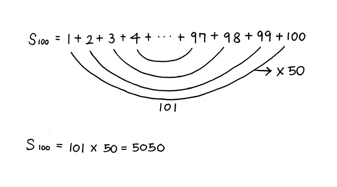
First, write down the numbers for the sum of 1 to 100.

Do you notice anything?

When we add 1 and 100, we get 101. When we add 2 and 99, we get 101.

And yes, the same applies to 3 and 98, 4 and 97, 5 and 96, and so on.

Apply this rule to the rest of the numbers and consider how many pairs of numbers in the series equal to 101 when added.

Do you notice how there are exactly 50 pairs?

Now, since we know all the details, all we have to do is multiply the two together.

When we do this, we get 5050. Therefore, the sum of 1 to 100 is 5050.

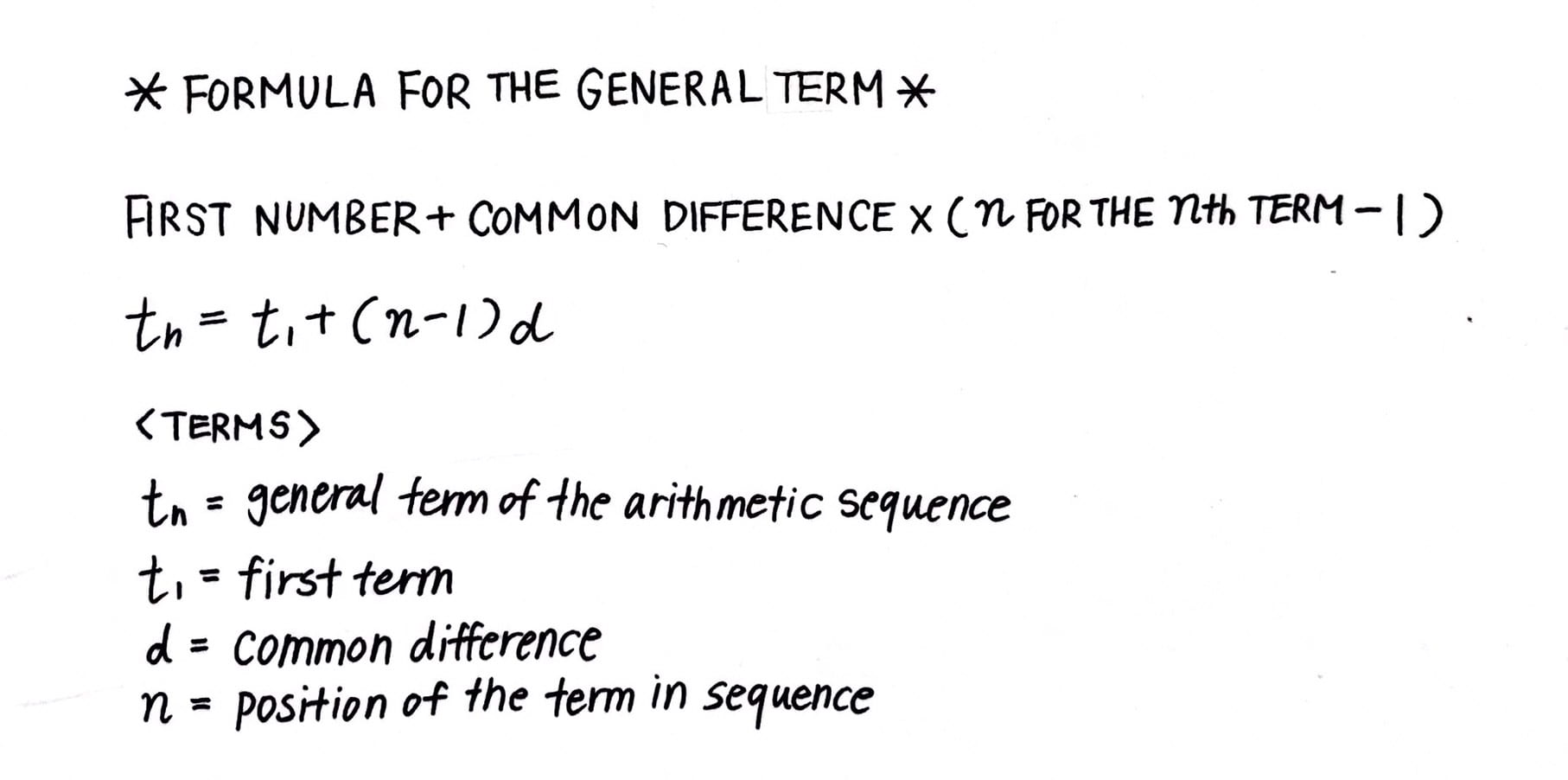
There is a formula used to find the sum of an arithmetic series.

It is basically the explanation above, but in a more simplified form.

You must add the first and last number of the series together and multiply it by the number of numbers in a series divided by 2.

That is it for this week’s post, and I hope this helped with your understanding.

Week 16 – math 10

ARITHMETIC SEQUENCES

This week, we learned about arithmetic sequences.

Let’s take a look at types of sequences and how to write the formula for the general term.

There are three types of  sequences: arithmetic, geometric, and other sequences that are neither arithmetic nor geometric.

In this unit, we will be dealing with arithmetic sequences.

The difference between two numbers in an arithmetic sequence is called the common difference.

It can also be written as d.

We can also write a formula for the general term of arithmetic sequences.

I hope this helped with your understanding of arithmetic sequences.

Week 15 – math 10

METHODS FOR SOLVING SYSTEMS OF EQUATIONS

This week we learned about the different methods for solving systems of equations.

Let’s go over what we have learned.

There are four ways of solving : inspection, graphing, substitution, and elimination.


INSPECTION

Inspection can be used when the equations are simple and able to be solved just by looking at them.

This method is time consuming and difficult to use when you are dealing with rather complex equations.


GRAPHING

Graphing makes it easy for you to find the solution of the equations because all you have to do is find the intersecting point of the two lines of the equations.

However, the points may result in decimals and if you wish to make it simpler, you may use the following two methods.


SUBSTITUTION

Substitution is the algebraic method that requires the act of substituting (that is, putting something in the place of another) to solve the equations.

It is a relatively quick method compared to the two above.


ELIMINATION

Elimination is the quickest way of solving equations so far.

It is used when all of the variables in the system of equations have a coefficient that is not 1.

You may either add or subtract the two equations to eliminate one of the variables in an equation.

This method saves you time and effort in the process of solving an equation.


I hope this helped with your understanding of the topic.

Week 14 – math 10

SYSTEMS OF EQUATIONS

This week we learned about system of equations and how to tell the number of solutions there are.

Let’s go over what we have learned.

When graphed, the lines help figure out how many solutions there are.

Even if not graphed, you can tell by looking at the slope and intercept of the equation.

Here is an example question. Let’s try and solve it together.

The answer is $2 for a cupcake and $1.5 for a cake pop, and it has one solution.


I hope this helped with your understanding.

Week 13 – math 10

DIFFERENT FORMS OF LINEAR EQUATIONS

This week we learned about the different forms of linear equations.


The three major forms of linear equations are the slope y-intercept form, the point-slope form, and the general form.

We write each form in the three following ways.


Slope y-intercept form : y=mx+b

Point-slope form : m(x-x1)=y-y1

General form : ax+by+c=0


The slope y-intercept form has m for its slope and b for its y-intercept.

It is used when given the slope of a line segment and the y-intercept.

For example, if given m=2 and (0,8), the equation in slope y-intercept form would be

y=2x+8


The point-slope form has m for its slope and (x1,y1) for the point of a line.

It is used when given the slope of a line segment and the coordinates of any point that is on the line.

For example, if given m=4 and (3,6), the equation in point-slope form would be

y-6=4(x-3)


The general form has a, b, and c for its constants.

In a general form, a, b, and c are integers, and a is a positive number.

For example, if given y=5x+24, the equation in general form would be

5x-y+24=0


I hope this explanation helped with your understanding of different forms of linear equations.

Week 12 – math 10

THE SLOPE FORMULA

This week, we learned about slopes, collinear points, and how to tell if line segments are parallel or perpendicular.

Let’s go over the things we learned from this unit.


First off, we have the slope of a line segment.

The slope of a line segment is the steepness and direction of the line measured.

We can also say it is the ratio of rise over run. (We will be dealing with these terms shortly after.)


You may be wondering, if the slope is the steepness of the line on the graph, what would the measurement of a vertical or horizontal slope be?

A horizontal slope can neither be positive nor negative, so the measurement of a horizontal slope is zero.

A vertical slope can be both positive and negative, so the measurement of a vertical slope is undefined.

A positive line segment rises from left to right.

A negative line segment falls from left to right.


Then we have the rise and run, which help with the calculation of the slope.

We can measure the slope of a line segment with the following equation : m = rise/run

The rise is the change of y , and the run is the change of x.

The rise is positive if we count up, and negative if we count down.

The run is positive if we count right, and negative if we count left.


Now let’s take a look at collinear points and parallel and perpendicular lines.


We can tell if points on a graph are collinear if they all fall on the same line.

This also means that collinear points all have the same slope.


We can tell if two line segments are parallel or perpendicular by taking a look at their slopes.

The line segments are parallel if they have the exact same slope.

The line segments are perpendicular if the result of the multiplication of the two slopes is -1.

[ Important note : If the line segments are perpendicular, keep in mind that each slope is the negative reciprocal of the other. This is valid if neither slope is equal to zero. ]


I hope this helped with your understanding about slopes.

Week 11 – math 10

THE DISTANCE AND MIDPOINT OF FUNCTIONS

This week, we learned about distance and midpoints and how we can tell how long the distance of a line segment is, and what the midpoint is.

Let’s start with vertical lines and horizontal lines.

Here are a few examples to help with your understanding.

Then we have the nonvertical lines.

Keep in mind that the distance should always be a positive number.

(If you got a negative number for the answer, simply get rid of the minus sign and make it a positive number.)


I hope this post helped with your understanding.

Week 10 – math 10

FUNCTION NOTATION


This week, we learned about function notations and graphs of functions.

First, let’s take a look at mapping notations, function notations, and equations.

In the form of function notation,  f  is the “name” of the function.

The input / independent variable is x, while the output / dependent variable is f(x).

[ Important note : Make sure not to make any mistakes while dealing with function notations. f(x) is NOT f times x , but rather an expression for “f of x” which means “function of x” ]


Now let’s look at several graphs and try to determine whether it’s a function or not by using the vertical line test.

You can run a vertical line through the graph, checking to see if there is more than one point on the same line. If there is another point on the vertical line, the graph is not a function.

For a relation to be a function, there must be only one output for each input, which in other words, means that there must be only one y value for each x value.

Therefore the last two graphs shown above are not functions.


I will post more information on my blog next week.

Week 9 – math 10

FUNCTIONS

This week we learned about functions and how to tell if a relation is a function or not.

Functions are considered special relations, where each input has only one output.

Therefore, they are categorized as relations.

Here are some examples of  how to tell if a relation is a function or not.

It comes to the conclusion that if you have only one output for each input, it is a function,

and if you have multiple outputs for an input, it is not a function.

It is the same with other graphs too, and you can easily notice if it is a function or not by figuring out if there is a chance of  y to have two or more values.

I will post more information next week.