Week 9 – Pre Calc 11 – Predicting the vertex

This week we learned how to predict the vertex of an equation without graphing it. We have not yet learned the equation to finding the vertex, but predicting the vertex lets us use what we know about quadratic equations without havinv to usw graphing technology. I chose this subjet because I find it to be straight forward and logical. This understanding is important because being able to indentify the vertex is a skill that will be used in math as we continue to develop our skillset.

Lets look at examples a and b that have been handwritten.

We can verify these solutions using graphing techonology to ensure we are correct.

Example C

Verify with desmos

Glossary :

Vertex – the maximum or minimum point on the equation’s parabola.

Parent function – x^{2}

Vertical translations – how far up or down along the y axis the vertex will be.

Horizontal translations – how far right or left along the x axis the equation will be.

Week 8 – Pre Calc 11 – Identifying whether a table of values represents a linear or quadratic function

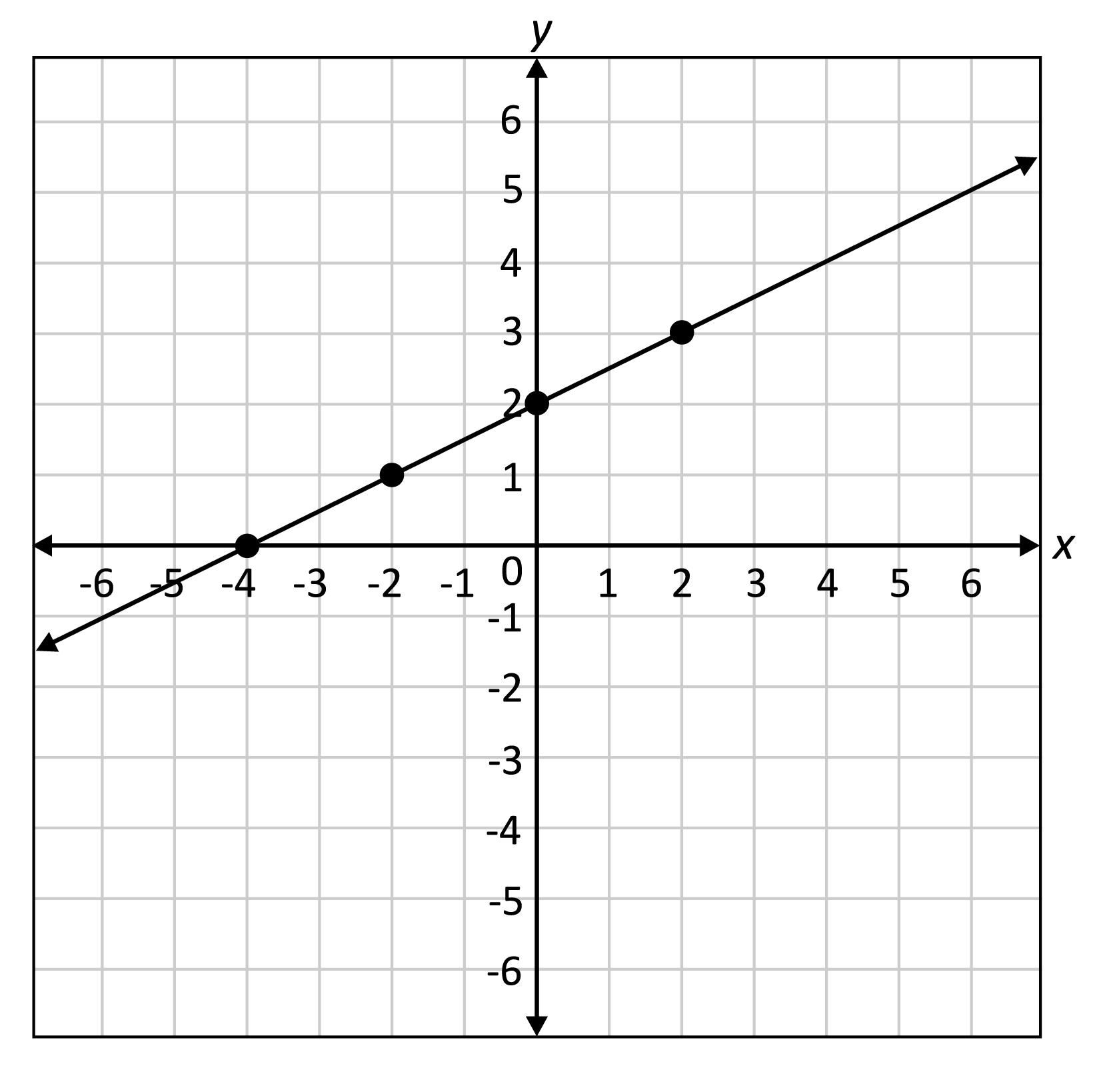
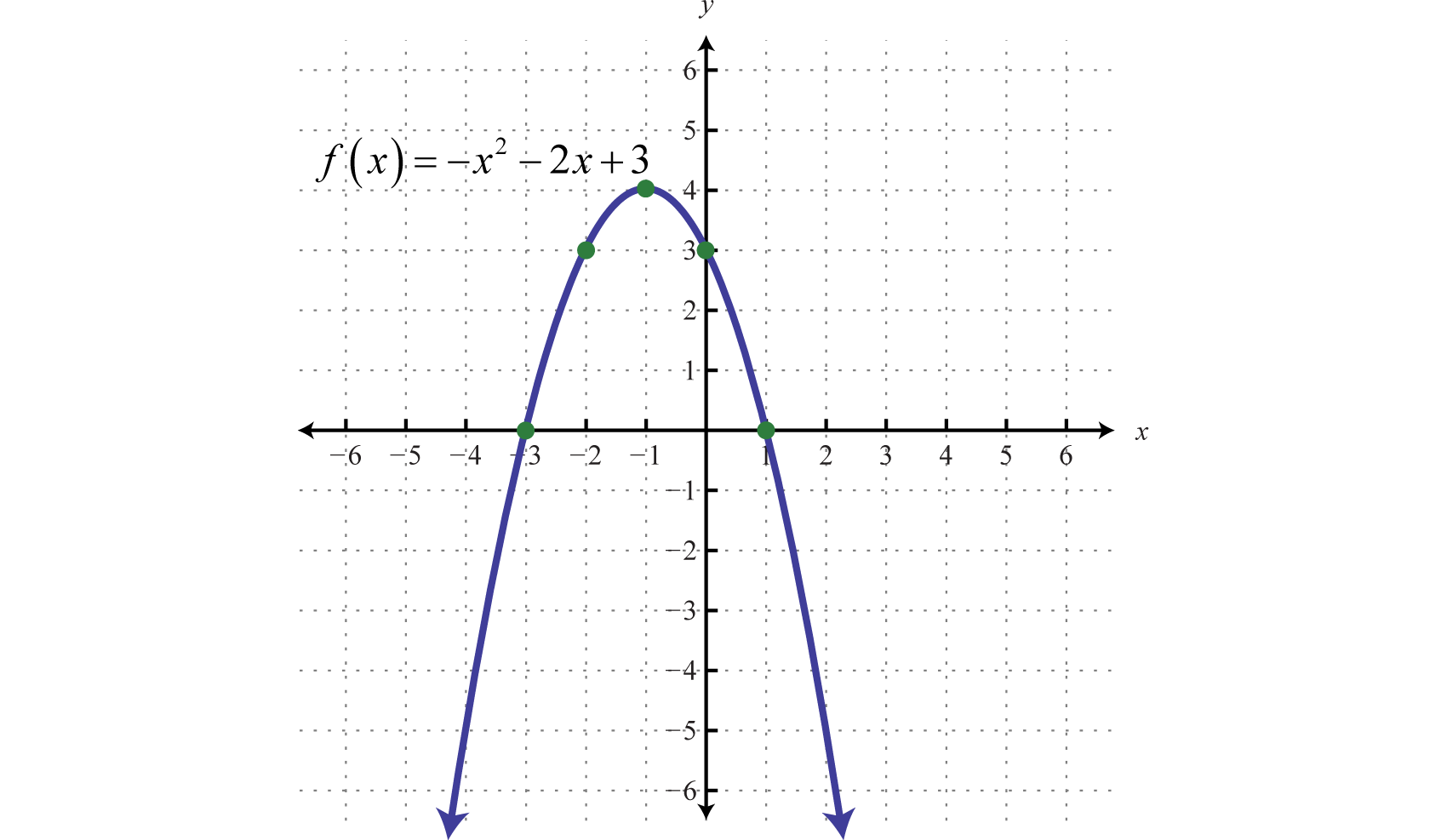
This week in math we learned the begging steps of graphing a quadratic equation, but before we learned how to do that we learned how to indentify if a function is linear, quadratic, or neither using a table of values. I chose this subject because I like having a visual, such as a table of values, to see what my function would look like. This understanding is important because knowing the difference between a linear equation, which we dealt with in earlier years, and a quadratic equation, which we are dealing with now and will continue to reappear in later math, is a fundemental skill and comprehension to have. For reference, lets look at a linear function on a graph and a quadratic function on a graph.

Linear :

Key Features of Linear Function Graphs (Sample Questions)

Quadratic :

Quadratic Functions and Their Graphs

Example a.)


Step 1. My first step is to observe the pattern of x values in my table of values, notice how they are decreasing by 1. Therefore, the difference between the y values may determine the behaviour of the ordered pairs.

Step 2. Find the difference between the first two terms. -2 – (-3) = 1. Repeat this process to find the first difference. You should get 1, 2, 4, and 8. Notice how the first difference is not constant. This indicates we are NOT evaluating a linear function.

Step 3. We can now find the 2nd difference. Use the values of the first term to find the second difference. The first value is 2-(1) = 1. Repeat this process and get 1, 2 and 4. Notice the second difference is NOT constant. this means that it is NEITHER a linear function or quadratic.

Example b.)

Step 1. Notice that the x values are increasing by 2 units. The difference between the y values may detrmine the behaviours of the ordered pairs.

Step 2. Find the first difference. To get our first value, find the difference between 5 and 0; 0 -(5) = -5. If you continue this process for the rest of the values you get -5,-7,-9,-11. Notice how the first difference is NOT constant meaning that it is not a linear function.

Step 3. Find the second difference. Use the values of the first difference, and find the difference between each value. -7 – (-5) = -2. If you continue this process you get -2, -2, -2. The second difference IS constant meaning it is a quadratic function.

Glossary :

Linear function :a function whose graph is a straight line, that is, a polynomial function of degree zero or one.

Quadratic function : the polynomial function defined by a quadratic polynomial.
Photo links :

1,700 × 987

1,640 × 1,638


Week 7 – Pre Calc 11 – Solving Quadratic euqtions with quadratic formula

This week in math we learned the quadratic formula and how to solve quadratic equations with this formula. I chose this topic because I find using the quadratic formula to be much more consistent and straight forward than ‘complete the square’ method. This skill is important because solving quadratics, especially with the quadratic formula, is a topic that we will build of off in our next units, and the next math courses that I will take.

Lets look at some examples…

Example 1.

This example is a simple quadratic without a leading coefficent larger than one.

Step 1. My first step is to write out the quadratic formula, so I can refer to it in my next step.

Step 2. In my second step, I need to identify the a,b and c values so I know where to plug in my values. In this particular example, the equation is already in general form which makes things much more simple. The X^{x} is my a value, the x is my b value, and my constant is my c value. This is how it always is.

Step 3. Plug in your a,b,c values into the quadratic equation to solve for x1 and x2. Remeber, if you have two negatives it is equal to a positive so -6 = 6.

Step 4. Expand your values

Step 5. Simplify the inside terms

Step 6. Simplify \sqrt{20}. 20 breaks down into 4 and 5, and because 4 is a perfect square, it comes out as 2.

Step 7. Since all terms are divisble by 2, we simplify and divide each term by 2. All terms must be divisble by the same value.

Example 2.

In this example we have a quadratic equation with a leading coefficent larger than 1.

Step 1. Convert the equation into general form. The -7x changes to a positive when it is moved to the other side of the equal sign.

Step 2. Identify values of a,b,c. Recall how we solved for these values in example 1.

Step 3. Plug each value into the quadratic formula.

Step 4. Expand the inside terms. BE CAREFUL. 4 X – 1 = -4; -4 X -4 = POSITIVE 16.

Step 5. Add like terms.

Step 6. see if you can simplify the radical, in this case we cannot which gives us our final answer. The +/- sign before the radical indicates there is two different answers. One positive and one negative. A quadratic equation always has 2 answers.


Glossary :

Constant :a number on its own, or sometimes a letter such as a, b or c to stand for a fixed number.

General Form : A formula that contains the degree of variables in decreasing order that = zero

Leading coefficent : the coefficient of the term of highest degree in a given polynomial.

Quadratic Equation : any equation containing one term in which the unknown is squared and no term in which it is raised to a higher power.

Pre Calc 11 – Week 6 – factorable expressions containing functions

This week in math we learned how to evaluate factorable expressions that contain functions, containing variables like x and y. This process is important because it allows you to solve for the restrictions of the variables as well the skill of being able to turn a complicated expression into a more neat and clean looking expression. Being able to factor expressions containing functions is important because it is a concept that we will build upon in further units and levels of math. I chose this topic because I enjoyed the process of substituting my functions with variables.

Lets look at some examples…

Example 1.

My first step is to rewrite the expression by subsituting variables where my functions are. Once you do this, you will notice my new expression is similar to the expresson a^{2} + 4a + 3

Now that I have rewritten my expression, I need to find what multiples of 1 and 3, multiply  together to give me a sum of 4. In this case, 3 x 1 = 3; and 1 x 1 = 1 | 3 + 1 = 4 which is what we needed to determine the factors of our expression. We add the terms across giving me (1a + 3) and 1a + 1) or in other terms (a + 3)(a + 1)

Now we want to subsitute our original values of x into a. (X + 2 + 3)(X + 2 + 1)

Finally we can add like terms, since 2+3 = 5 the first factor is (x + 5) and our second factor is (X + 3)

Example 2.

In my first step, I substitute my functions of x + 2 and y + 5 with a and b; x + 2 = a; y + 5 = b

In my next step, I look for one thing in common between both terms. I divide 32 and -18 by the GFC of 2.

In this step, I move the two that I simplified the expression with outside of the brackets, you cannot get rid of it. This leaves me with 2(16 a^{2} – 9 b^{2})

I can further factor this expression because 16 and 9 are perfect squares, and a^{2} and b^{2} means that there is one a and one b in each set of brackets. This leaves me with  2(4a + 3b)(4a – 3b)

5. In this step, I subsitute my original functions back into my factored expression 2(4a + 3b)(4a -3b) = 2[4(x+2) + 3(y+5)] and my second term [4(x+2) – 3(y+5)

6. Now I can expand this expression and collect like terms. Distribute 4 to x + 2. 3 to y + 5. On the right side i do the same, distribute 4 to x and 2, and -3 to y and 5. My new expression is now 2(4x + 8 + 3y + 15) and on the right side (4x + 8 – 3y – 15)

7. Finally I can add like terms giving me 2(4x +3y + 23)(4x -3y -7)

Glossary:

Function : A function from a set X to a set Y assigns to each element of X exactly one element of Y.

subsitute: substituting the value of any one of the variables from one equation into the other equation.


What Darwin Never Knew – Life Sciences 11

Question : How did the discovery of DNA prove that Darwin’s theory of evolution was correct and how does it change the way we view evolution today and into the future? 

Darwin made his start on discovering the theory of natural selection on his five-year voyage on HMS Beagle from 1831 to 1836. HMS Beagle - WikipediaOn September 15, 1835 on the return route across the Pacific, the Beagle arrived in the Galapagos Islands where Darwin would make his most notable discoveries. It was here on the Galapagos, that Darwin discovered the vast diversity of different animals on the islands, some species being exclusively located on the Galapagos, such as the finches he discovered.Origin of the species: where did Darwin's finches come from? | Birds | The Guardian He noticed that different finches differ in the type of beak, depending on the island and how different tortoise species lived on islands with different environments, and that there were differences in their shells depending on their location. Darwin drew the conclusion that some species happen to change. Darwin began his study of dog breeder’s and how they were able to breed different dogs together to obtain a specific trait. All the evidence Darwin gathered led him to drawing his theory that ‘species can change over time, that new species come from pre-existing species, and that all species share a common ancestor.’ (khanacademy). 

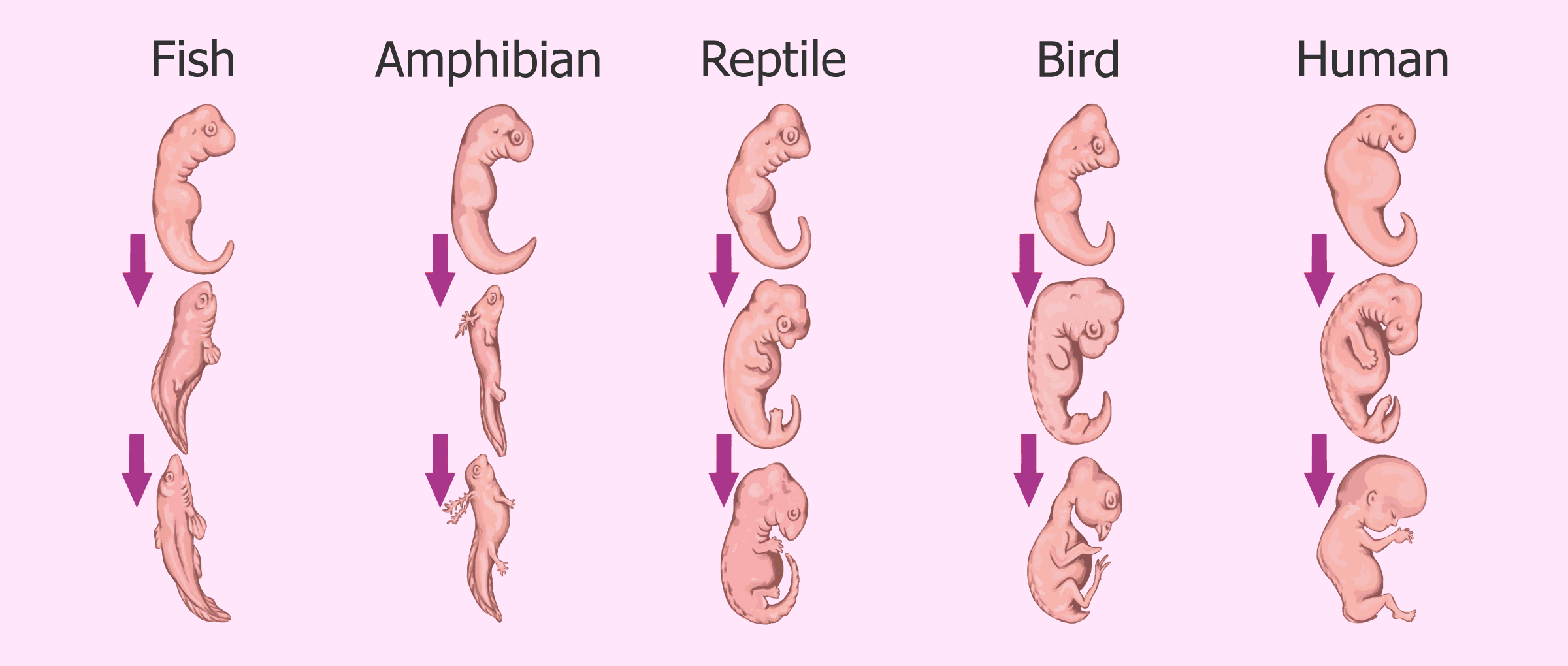
     There were various pieces of evidence for Darwin’s theory of evolution at the time such as that of fossils. Fossils are preserved remains of organisms, often found in sedimentary rock. Fossils provide a record of how organisms evolved. nationalgeographic). hThis process of evolution can be visualized as a ‘tree of life’, showing that all species are related to eachother at a common ancestor, but branch off and evolve into different species. However, Darwin’s theory of natural selection, would be further solidified in 1953 with the discovery of the double helix DNA, by researchers James Watson and Francis Crick. With further investigation, it was discovered that many genes of DNA get translated into proteins that make up our bodies, and that DNA does not stay the same. This proves his theory that organisms are changing, and that there is a linear pattern that traces back to one common ancestor. DNA explains the patterns seen in homologous structures and provides even more evidence for Darwin’s theory of evolution. Some homologous structures can only be observed in the embryotic stages of development, but upon closer look, many organisms such as fish, humans, and birds share a similar homologous structure during the embryotic stage of development. Human embryo compared to other animals(biologyonline). For example, all vertebrate embryos have gill slits and a tail during early stages of development. The developmental patterns of these species begin to differ as development advances, which explains why the embryonic tail of a human is now a tailbone, and the ‘gill slits’ develop to become into the jaw and inner ear. These shared features suggest that all living things descend from a shared ancestor, and that this ancestor had DNA as its genetic material, used the genetic code, and expressed its genes. The reason that we do not still have our tail, and why we differ from birds or fish is due to Mutation. Hox genes encode transcription factors and are necessary during embryonic development for determining how the cells in a specific region develop, however all that is needed to determine if an animal has arms, or gill slits is a few mutations. This process entails a piece of DNA called a ‘switch’ that turns “on” or “off” genes. (What Darwin Never Knew). Genes are turned on and off in different patterns during development to allow for the differentiation of cells. This connects back to Darwin’s theory of evolution because it the reason that all species of life are related but evolve to become different. A great example of how mutations coded for a new species is that of many prehistoric fish, specifically that of the Tiktaakik.Started Out as a Fish. How Did It End Up Like This? - The New York Times (What Darwin Never Knew). It has the body of a fish with scales, but also the bone structure is seen in all four-legged forms. The fish evolved into what we know as modern-day land animals. However, some of the same bone structure remains between fish and land animals such as human. Another example is the biological composition of human and chimps. Chimps are human’s most closely related relative, with only a 1% difference in DNA. (What Darwin Never Knew) Once again, mutation is responsible for the evolution into different species. After the separation of ancestor lineages, human and chimpanzee genomes experienced various mutations such as single nucleotide substitutions, deletions, and duplications of DNA fragments of different size, insertion of transposable elements and the rearrangements of chromosomes. (Live Science). Differences in the sequences of DNA that turn genes on and off, and through sequences of the DNA that throw switches, is what is responsible for the large changes of different organisms, despite only small differences in the DNA molecule itself.  This shows how small differences in DNA can generate enormous change. 

      Today we view evolution as an accepted part of science, as the process of gradual change that takes place over many generations where traits are passed from parent to offspring (nature). Darwin can be credited for pushing to dismantle the idea that all organisms on earth are created by God, but rather have evolved over time and come from a common ancestor. Darwin’s theory along with the discovery of DNA provides a strong foundation for the future study of evolution. With the discovery of DNA, our understanding of genetic mutations such as microcephaly, will continue to revolutionise science and will aide in solving some of the greatest mysteries to date regarding evolution and DNA as science advances.

Sources :

https://www.nature.com/scitable/definition/evolution-78/

https://www.khanacademy.org/science/ap-biology/natural-selection/natural-selection-ap/a/darwin-evolution-natural-selection

https://education.nationalgeographic.org/resource/fossil/

https://www.biologyonline.com/dictionary/homologous-structures

https://www.livescience.com/15297-chimps-humans.html

Youtube : ‘What Darwin Never Knew”


Week 5 – Pre Calc 11 -Solving equations algebraically

This week in math, we learned how to solve radical equations using algebra. This is important because solving equations graphically is not always the most accurate or efficent. Using algebra to solve equations gives us a more precise, step-by-step approach to solving for our variable. I chose this topic because using algebra provides a strong visual as to what is happening throughout each step of solving the equation.

Let’s look at some equations to solve…

Example 1.

Step 1. In my first step, I recognize that their is a binomial on the left side of my equation. My goal is to isolate for x, and the first step in isolating x is turning this bionomial into a monomial. To cancel out my coefficent of 6, I can add -6 to each side of the equation, because what you do on one side you must do on the other side. 10 – 6 = 4 which gives me my value for the right side of the equation.

Step 2. In this step, I want to free the radicands from the square root sign, by squaring it. Square rooting and squaring are opposites, so this cancels out my root sign, leaving the terms on the inside the same. Once again, what we do on one side of the equation we must do to the other side, so we square 4 as well 4^2 = 16.

Step 3. In this step I am left with x – 3 = 16, but remember we want to isolate x, so we must add +3 to cancel out the -3 on the left side, and do the same on the right side, adding 3 to 16. Finally we have solved for x, giving us ‘x = 19’

Step 4. Verify! It is important to understand how to verify that your solution is correct by substituting it back into the original equation, to avoid an extraneous root. Since we know x =19, we plug it into the x value. \sqrt{19-3} gives us \sqrt{16}. We know that \sqrt{16} = 4 so now we cam combine our coefficent (6) with 4. 6 + 4 = 10 which matches our value on the right side of the equation (10 = 10,) our solution is correct!

Example 2.

In this example their is a fraction involved, which can look confusing when solving for x. However, we can use what we know with fractions to get rid of it.

Step 1. I know that the opposite of division is multlipication, so I multiply 5 on both sides of my equation to cancel my denominator of 5. That leaves us with \sqrt{14x-3}= 10.

Step 2. Now that we have gotten rid of our fraction, we can go about the equation like normal by canceling out the square root by squarting it, and doing the same on the right side of the equation as well. This gets rid of our root sign, and since we are squaring 10, we get 100 (10^2 = 100)

Step 3. Now we want to further isolate x. We can go about this by canceling out -3 with +3, and +3 is added to the right side which gives us 4x = 103.

Step 4. To get rid of the coefficent 4, which is infront of x, we divide both sides by 4. This gives us x = 103/4

Step 5. Verify! We need to plug 103/4 back into the x’s place. Luckily, since the original equation has coefficent 4, the denominator of 103/4 is canceled out. Now we can subtract \sqrt{103-4} which = \sqrt{100} / 5. The square root of 100 is 10, divided by 5 = 2. Which means 2 = 2, our solution is correct!


Glossary :

Extraneous root – values that we get when solving equations that aren’t really solutions to the equation.

Isolate for x = get the variable ‘x’ on its own.

Solution : A value or values which, when substituted for a variable in an equation, make the equation true

Substitue / substitution : Used to solve the system of equations it is like ‘plugging in’ your solution into the variable’s place.


Week 4 – Pre Calc 11 – Adding / Subtracting Radicals with radicals

This week in math we learned how to add and subtract like radicals. I chose this topic because I like the process of breaking down entire radicals to reveal their radicands which are used to determine if different radicals are like terms. This process is crutial in understanding the rules for how different values can be grouped together and simplified, or must be left untouched if the value has no other like terms. Being able to make the connection that radicals with the same radicands are like terms is an important concept to understand in further our understandings of mathamatics.

Lets look at some examples…

  1. In the first example I used a subtraction question with binomial. In my first step I recognize that 20 breaks down into 4 and 5. This is great because I am looking for perfect squares, and since 4 is a perfect square I can move its square root (2) into the coefficents spot. 125 breaks down into 25 and 5, since 25 is a perfect square its square root (5) can move into the coefficents spot, and the 5 that is left over from 25 and 5 stays in the radicands spot because 5 can not be further simplified, it is prime.
  2. Next we deal with the variables. Notice that in 2 \sqrt{5x^5y^4} there are 5 copies of x and 4 copies of y. Because we are evaluating a square root, we are looking for groups of 2 we can pull out of the radicands spot and into the coefficent spot. Five copies of x means we can take out four x’s which comes out as 2 x’s or x^{2}. There are four y’s so we can take out all four which becomes y^{4} in the coefficients place.
  3. After simplifying both terms we are left with two of the same radicands ‘\sqrt{5x}‘ which means they are like terms and we can add or subtract the coefficents.
  4. Because we are subtracting I am looking for like terms that can be simplified but since 2,  x^{2} and y^{2} are all unlike terms they are already simplified to the most they can be. This leaves us with 2 x^{2} y^{2} – 5y and \sqrt{5x}. This is the most simplified \sqrt{20 x^5 y^4}\sqrt{125 x^2 y} can be.

\sqrt{20 x^5 y^4}\sqrt{125 x^2 y} = (2 x^{2} y^{2} – 5y) \sqrt{5x}

This next example will be a bit longer so lets look at the steps we can take to evaluate it.

My first step is to break down each root into mixed form. I can break down \sqrt[3]{16x^5} into 8 and 2 and because 8 is a pefect cube it moves into the coefficents place as 2 (cube root of 8 is 2). The variable v has 5 copies, within the 5 we circle 3 v’s which comes out as v in the coefficents place with 2 v’s left in the radicand spot that cannot be further broken down. I can also break down \sqrt[3]{24w} into 8 and 3. 8 becomes the coefficent and the 3 is left as the radicand with w left in the radicand because it cannot be further broken down. Same process with -5v \sqrt[3]{54v^2}. I can break down 54 into 27 and 2, I do this because I am looking for perfect cubes, and 27 is a perfect cube. I can move 27 into the coefficents place as 3 ( \sqrt[3]{27} = 3 ) and the 2 and v^{2} are left in the radicands place because they cannot be further broken down. The reason we left  \sqrt[3]{3w^4} alone is because it cannot be further broken down. This means it has an inivisible coefficient of 1.

In my next step, I have written all my terms as mixed radicals in their most simple form. I notice that out of the 4 terms, 2 have a radicand of 2v^{2} and 2 terms have the radicand 3w.  For the terms with the radicand 2v^{2}, I can add their coefficents which gives me -13v (2v-15v = -13v). The coefficents with the radicand 3w become 5w (w + 4w =5w)

For my last step I put my two terms together to get -13v \sqrt[3]{2v^2}  + 5w \sqrt[3]{3w}

We must also indentify the restrictions of the variables V = R ; W = R because they both are under cube roots.


Glossary :

a binomial is a polynomial that is the sum of two terms

Like terms: Terms that contain the same variable which is raised to the same power.

Prime : a whole number greater than 1 whose only factors are 1 and itself.

Pre calc 11 – Week 3 – Simplifying roots with variable radicands

This week in math we added to our understanding of knowing how to evaluate roots, but instead of evaluating roots that have intiger radicands, we learned to how to break down a variable radicands such as ‘x’ or ‘a’ or ‘y’ or whatever the variable may be. I chose this subject because I learned how to visualize the process evaluating roots in a much more indepth way. This visualization applies to evaluating all roots and is something that I will take with me as I progress in pre calc 11,12 and calculus. Prior to Pre Calc 11, I felt intimidated by variables in math, seeing numbers and letters all mixed together often confused me but it is never as complicated as it seems if you learn the right approach. This skill is important because it is a reoccuring topic in math will advance.

Lets look at one example of evaluating roots with variable radicands.

In my first step, I broke down \sqrt{x} into \sqrt{x . x . x . x . x . x . x} because really, the index 7 is telling us there is seven copies of x!

In my next step I am looking for groupings of 2, because it is assumed that we know a square root’s index is an invisible 2, therefor we look for factors of two of the same value, in this case it is the variable x. In each set of two X’s, we only need one of the two when we move these groupings into the coefficent place. Whats left is the X that does not have a partner or another one of its self that it can group two, so we leave it where it is under the root sign in the radicands spot.

In my last step I put all of this information together to get x ^{3}  or in other words three copies of x. Make sure that when you are writing out your exponent of x that you don’t confuse it with your index!

Example 2.

To start off, we need to recignize that we are evaluating a cube root, that is why I circled the index ‘3’ and labeled it so we do not forget. That means we are looking for groups of three.

In my next step, I recognize that x ^{4} tells me that there are four copies of x. I like to write out all 4 x’s to better visualize this.

In my next step, I know that we need to find 3 x’s that we can group together as 1, because when dealing with cube roots, we are looking for groups of three of the same value. This leaves us with one x  left over that is not apart of the circled 3 x’s. This x is what stays under the root sign because it has no where else to go, it is unique and alone as the radicand. Our one group of three x’s however can be moved into the coefficent place to indicate that within our root there is a perfect cube (the three x’s).

Step 4. I put all of this together to get my final answer. Remeber however that in this example our index is three and not the exponent of x.

Glossary:

Coefficent : A number used to multiply a variable.

Exponent : the number of times a number is multiplied by itself (how many copies of its self there are)

Variable : an unknown numerical value written as a letter.


Week 2 – Pre Calc 11 – Writing powers as radicals

This week in math we learned how to write powers as radicals in which we can evaluate or write them as a mixed radicals. The powers that we’re dealing with in this unit are written in fractional and decimal form which at first can make things look confusing. I chose this topic because evaluating fractional powers is a concept that I was previously unfamiliar with, however I have grown to find the topic fascinating and and a very logical straight forward process. This skill and understanding will be important to know for furthering our understanding of powers and roots.

To start, let’s learn how to convert an exponent that is in decimal form into fractional form (it makes writing powers as radicals much easier).

Example 1.

Step 1. Convert the exponent into fractional form. To do this, you need to consider place value; the denominator of the fraction will be the place value. The digits of the decimal will equal the numerator. In this case we can write the numerator 1.5 as 15. The denominator is written as 10 because the 5 is in the tenths place. The new fraction can now be written as \frac{15}{10}. Next we simplify the fraction by the GCF to clarify communication and to avoid misunderstandings. In this case the highest value that 15 and 10 can be divided by is 5; the new fraction is now \frac{3}{2}.

Step 2. We now convert the base of our power (0.25) into fractional form. Similar to converting the power, 0.25 can be written as \frac{25}{100} because the place value is in the 100th. We must now reduce this fraction once again to reduce the odds of any other misunderstandings. The GCF is 25 because it can evenly divided into 100 and our new fraction in its simplist form is \frac{1}{4}.

Step 3. Lets put together our simplified exponent and base to get the power in fractional, simplfied form. The new power is 1/4^{3/2}

Step 4. In order to convert our new power 1/4^{3/2} into a radical we must recognize that the denomator of our fractional exponent is the index, and the numerator is written as the exponent  in radical form.

Step 5. The method I find to be most efficent is to evaluate starting with the index before I distribute the exponent. Knowing this, \sqrt{1} = 1 and \sqrt{4} = 2, because as we have learned a factor of a number that, when multiplied by itself, gives the original number; 2×2 gives our original number,4. Now we can distribute the exponent 3 using in relation to the power law.

Step 6. In other words, the exponent 3 means that there is 3 copies being made of \frac{1}{2}. 1 x 1 x 1 = 1 and 2 x 2 x 2 = 8. The final simplified answer is 0.25^{1.5}\frac{1}{8}.

Example 2.

In this example, you will find that it cannot be fully evalauted, so instead we can convert it into a mixed radical.

Step 1. Just like in the first example, we can turn the power into radical form by using the denominator of our fractional exponent as the root and the numerator as the exponent. This time there is no decimals to convert. However, upon writing our power in decimal form we can immediately see that (-16) is not a perfect square so we must distribute the exponent 2 to (-16) instead.

Step 2. Distributing the 2 to (-16) affects everything within the brackets; in other terms it means there is two copies of (-16). Two negatives = a positive, so we can look at this expression as being the same as positive 16^{2}. I solved this equation by using long multiplication; this removes the need for a calculator. 16^{2} = 256.

Step 3. We also need to recognize that \sqrt[3]{256} is also not a perfect cube, so we must convert it into a mixed radical to further evaluate it. Firstly, we need to break down 256 using prime factorization. Because we are evaluating a cube root, we can circle and group together each set of 3 of the same value. In this case I circled 2 groups of three 2s. Then, we can move these twos into the coefficient position of the radical. We only need to take one 2 from each group, the rest cancel out. As our coefficient place we now have 2 x 2 or 4. The prime factors that are left, will be used as our radicand; this is 2 and 2 (2×2) which gives us 4 as our radicand. We put everything back into exponential form and we get 4^{3} \sqrt{256}.

Glossary

GCF (greatest common factor) – The highest number that divides exactly into two or more numbers.

Place value – The system in which the position of a digit in a number determines its value.

Power – An expression that represents repeated multiplication of the same factor

Power Law – exponent is being distributed to the value within brackets, multiplying with other exponents.

Prime factorization – a process of writing all numbers as a product of primes.

Prime number –  a whole number greater than 1 whose only factors are 1 and itself.

Week 1 – Pre Calculus 11 – Estamating Values of Radicals

This week I learned how to estimate the number value of two radicals (an expression containing a square root) that may not be a perfect square, perfect cube, or perfect fourts. In previous learning, evaluating square roots was exclusivly evaluating perfect squares such as \sqrt{25} which as we know is equal to 5, because \sqrt{25} in other terms is symplifying 5 to the power of it’s self. This week in math I was introduced to evaluating perfect cubes, such as \sqrt[3]{27} which is equal to 3, because the cube root of 27 is the number which when multiplied by itself three times gives the product as 27, since 27 can be expressed as 3 × 3 × 3. Therefore, the cube root of 27 = ∛(3 × 3 × 3) = 3. We have also looked at perfect fourths such as \sqrt[4]{16} which is equal to 2 ( 2^{4} ). But what happens when you need to estimate the value of a radical that is not a perfect square, cube, or even fourth?

These are the steps to go about it…

In the first example I am evaluating the cube root of 20, which is not a perfect cube. Therefore, the next best way to evaluate this cube root is to estimate it’s value to the nearest tenth, using what knowledge we have about perfect cubes. This is a crutial skill to have, as throughout pre calculus 11, evaluating radicals without a calculator is a re-occuring concept. Furthermore, I chose estimating the value of radicals as my subject for this week’s post because in the past I have struggled with understanding radicals as well as making mathematical estimations; however, I feel more comfortable now due to the homework we completed in class.

Further explanations of the steps from example 1.

Step 1- After memorizing the first 10 perfect cubes, I was able to recognize that 20 is not a perfect cube, and I must find the two perfect cubes 20 falls between in order to make an estimation on it’s value.

Step 2- I made the connection that 20 falls in between the two perfect cubes 8 and 27.

Step 3- I calculated the difference between 20 and 8 and 27 and 20. The cube root of 27 was closest to 20 which would mean my value has to be closer to \sqrt[3]{27}, which after evaluating we know that \sqrt[3]{27} = 3, and \sqrt[3]{8} = 2, in other terms \sqrt[3]{20} falls between 2 and 3 but is closer to 3.

Step 4. I know that my value is closer to 3 but cannot surpass it, so my educated estimate would be \sqrt[3]{20} ≈ 2.7


Example 2.

Further explinations of example 2

In this example I chose a value that was a bit larger, the square root of 116. I chose this value because usually larger numbers tend to intimidate people, including myself but the steps in evaluating this square root are actually quite simple.

Step 1- I recognized that \sqrt{116} is not a perfect square, as 116 cannot be expressed as the product of two equal integers.

Step 2- I know that in order to estimate the value of \sqrt{116} I need to find the two perfect squares that it falls between, which as we know are 100 ( 10^{10} ) and 121( 11^{11}).

Step 3- Calculate the difference between 116 and 100 and 121 and 116. You will find that 116 is closer to 121. We now need to evaluate \sqrt{100} = 10 and \sqrt{121} = 11. This means my value must fall between 10 and 11 but is closer to 11.

Step 4- I estimated my value to the nearest 10th and because the value is closer to 11, but cannot surpass it, my educated estimate is \sqrt{116} ≈ 10.8

Example 3.

Further explinations of example 3.

Step 1- Recognize that \sqrt[4]{79} is not a perfect fourth, it is not a number that is equal to being multiplied by itself four times. How do you know this? It takes a bit of memorization if you choose to do so; however, the perfect fourths can be learned by continuing the multlipication of perfect squares and cubes: (i.e. 2^{2} = 4 which is the perfect square, multiply 2 to the power of 3 for the perfect cube: 2^{3}  = 8 and 2^{4}  = 16 which is the perfect fourth.

Step 2- After listing out the first few perfect fourths, I saw that 79 must fall in between \sqrt[4]{16} and \sqrt[4]{81}. After finding our two perfect fourths, we must evaluate \sqrt[4]{16} = 2  and  \sqrt[4]{81} = 3.

Step 3- I calculated the difference between 79 and 16 and 81 and 79; 79-16 = 63 and 81-79 = 2. We have now indicated that \sqrt[4]{79} is significantly closer to the value of 3, but cannot surpass it.

Step 4- Educated estimate! \sqrt[4]{79} ≈ 2.9

Glossary

Perfect cube: a number that is multiplied by itself three times

Perfect fourth: a number that is multiplied by itself four times

Perfect square: the product of a rational number multiplied by itself

Power: (aka an exponent) is a number that states how many times you need to multiply the number by itself

Radical: The √ symbol that is used to denote square root or nth roots, it consists of the root symbol, the radicand (number within the root symbol) and when dealing with anything greater than perfect squares, an index which is a small number on the left of the square root tells us how many times a term has been multiplied by itself.

Square root: a number which produces a specified quantity when multiplied by itself