This week in Pre Calc 11 we learned about properties of Quadratic Functions. We learned how to determine the vertex of a Quadratic function and if it is minimum or maximum, the line of symmetry, the x and y intercepts, the domain and range and we also learned how to determine if a function is going to be congruent to the parent function:  Using all of these properties that we learned, we were then able to analyse Quadratic Functions written in Standard Form or as Mrs. Burton likes to call it Vertex Form, to later be able to graph them very easily. This is an example of a Quadratic Equation written in Vertex Form:
 ^2-6.") This Vertex Form is also known as
This Vertex Form is also known as ^2+q.") Knowing what each of the different variables represents in this form can help you analyse the function and allows you to get a really good sense of what it would look like on a graph.
Knowing what each of the different variables represents in this form can help you analyse the function and allows you to get a really good sense of what it would look like on a graph.
In Vertex Form, ^2+q") :
:
 is the vertical translation, which means that it will translate either a certain number of units up or down along the y axis. It also tells us what the
  in the vertex is going to be.
 is the horizontal translation, which means that it will translate either a certain number of units to the right or to the left, moving along the x axis. It also tells us the line of symmetry and what the
  in the vertex is going to be. However we must remember that the sign changes when you take the
  value out of Vertex Form and put it into your vertex. Example:
 ^2-6") the vertex for this function would be
the vertex for this function would be .")
 tells us the parabola is going to be congruent to the parent function, if it going to be a reflection or not and if it is going to be a stretch or a compression. If the value of
  is is a number other than 1, then the parabola will not be congruent to the parent function. If the sign is negative the parabola will have a maximum vertex, which means that it opens down and that it will be a reflection, however if positive the parabola have a minimum vertex which means that it will open up. If the value for is a fraction then the parabola will become wider and will be a compression and if the value is a whole number, then the parabola will become skinnier and will be a stretch. Example: in this function, the parabola will be a reflection, it will have a maximum vertex which means that it will open down and it is a stretch.
In the example ^2-6,") that I used throughout this post, we discovered that the vertex is going to be
that I used throughout this post, we discovered that the vertex is going to be ,") that it is not congruent, that it is a reflection and has a maximum vertex. If I were to graph this function with the information that I have determined, the function would look like this:
that it is not congruent, that it is a reflection and has a maximum vertex. If I were to graph this function with the information that I have determined, the function would look like this:


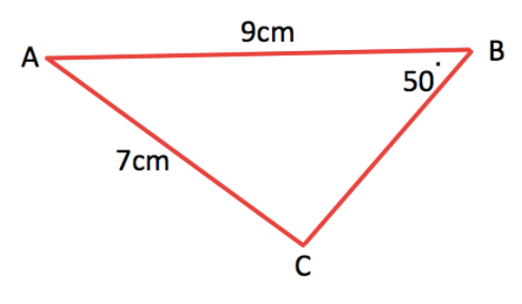


}{7}=sinC.")


 you would first want to move the
  to the right side of the equation to be able to solve it in a more efficient way, because they have a common denominator you are allowed to subract 3 by 2. Another way to solve rational equations is by cross multiplying. However, this method only works if there are only two fractions, one on either side of the equal sign. For exmaple,
  is an example of an equation that you are able to cross multiply to help you solve it. To cross multiply, you multiply
 (2)") and
and (x+4),") leaving you with
leaving you with =5x(x+4)") as your new equation. We also learned how to multiply through an equation using a common denominator. When you do this, you are putting the entire equation over a common denominator which means that it can basically cancel out when you multiply through, which will leave you with only the numerator to solve. For example,
as your new equation. We also learned how to multiply through an equation using a common denominator. When you do this, you are putting the entire equation over a common denominator which means that it can basically cancel out when you multiply through, which will leave you with only the numerator to solve. For example,  can be easily solved if you multiply each fraction by the common denominator which is
 .") This will leave you with
This will leave you with =4x.") Once we have cancelled out the numerator, you can now solve for
Once we have cancelled out the numerator, you can now solve for  The last method that we learned was that if the numerator’s or the denominator’s of an equation that has only two fractions (one on either side of the equal sign) are equal to one another than that means that the numerator’s or denominator’s must also be equal. This allows you to eliminate the numerator’s or the denominator’s to make it easier to solve. For example,
  have the same denomintor which tells you that the numerator’s will also be equal to one another, allowing you to eliminate the denominator’s, leaving you with a simplified equation of
  From there you must determine whether or not it’s quadraitc or linear and then you can solve for
  (\frac{2y}{3x^2})") I would first simplify the expression, by eliminating the
I would first simplify the expression, by eliminating the  from the numerator and denominator of this expression and I would also simplify the
  and
and  to become
  Leaving me with the newly simplified expression,
  (\frac{y}{3}).") Next we are able to multiply straight across giving us our final answer:
Next we are able to multiply straight across giving us our final answer:  This is our final answer because it can not be simplified any further.
 is
is  because the values flipped. In order to graph reciprocal linear functions we must first graph the parent function. Next we will be able to find the horizontal and the vertical asymptotes. In grade 11, the horizontal asymptote will always be drawn along the x-axis, which means the equation for our horizontal asymptote is
  To determine where the vertical asymptote will be, we must find where our parent function intersects the x-axis, which will be our x-intercept and draw a vertical line through it. This line will be our vertical asymptote, represented by
  Once we have determined our asymptotes, we now must find the invariant points. The invariant points are are determined by where the parents function crosses the numbers
  and
and  on the y-axis. We are now able to graph our reciprocal linear functions by starting at the invariant points and drawing two hyperbola’s that follow along the horizontal and vertical asymptotes, gradually getting closer to them, but never actually touching them.
 is has a slope of
  and it’s y-intercept is

 and
and  because as we can see in the graph, the x-intercept of the parent function is
 (0).") Next we must find the invariant points which will be
Next we must find the invariant points which will be ") and
and .") Finally, we are able to draw our two hyperbola’s.
Finally, we are able to draw our two hyperbola’s.
 the seperated equations would be:
  and
and  Next, we would graph both equations in order to visually determine how many possible solutions the absolute value equation might have and the vaules of the possible solutions. Linear absolute value equations can have 0, 1 or 2 solutions. We must also remember that since the equation has abosulte value bars around it, the equation can not be graphed in the negative zone of the graph and will instead reflect back up into the positive zone, making a V shape.
 and
and  This also shows us that this absolute value equation has two solutions.
 we must seperate the equations to be able to graph them. The sperated equations are:
  and
and  Next we graph both equations to determine their points of intersection. Quatratic absolute value equations can have anywhere from 0 to 4 solutions.

 and
and  This also shows us that this absoulte vlue equation has three solutions.
 we must first start by getting rid of the absolute value bars by putting this equation into two different equations using piecewise notation. This means that our two new equations will be
  and
and .") Once we have our new equations we must solve to determine the value for
Once we have our new equations we must solve to determine the value for  which will tell us how many times the eqautions will intercept. In the first equation:
  to the other side which gives us
  from there you continue to isolate
  In the second equation:
 ") we must follow similar steps, however we must first distribute the negative into the brakets before we can make the equation equal to zero. Once you isolate for
we must follow similar steps, however we must first distribute the negative into the brakets before we can make the equation equal to zero. Once you isolate for  This tells us that the equation
  the y-intercept is the second term which is positive
  and a run of
  We also learned how to determine whether the boundry line of the linear inequality will be broken or solid. If the linear inequality is greater than, less than or equal to (includes), then the boundry line will be solid, however if it is only greater than or less than (excludes), then it will be broken. For example in the inequality:
  the inequality sign tells us that the value for
  we know that the slope is
  the y-intercept is

 is our first term and that this sequence has a common difference of
  which means that in order to determine tha value of term 12 we will need to input the information that we already know into the equation
  =
= (d),") as I have shown in the example below.
as I have shown in the example below.
 or that
  If it is converging, it means that
  or that
  If the Infinite Geometric Series is diverging it means that it will have no sum, however if it is converging than you are able to caculate the sum.
.") It looks like this:
It looks like this: (x-x2).")
 and it also tells us if the parabola opens up or down. It looks like this:
 In this example you must first get rid of the coefficient by dividing the first two terms by three. Ex.
 =y.") Then you must find the zero pairs by dividing the middle term by two and then squaring it. Ex.
Then you must find the zero pairs by dividing the middle term by two and then squaring it. Ex. -72=y.") Then you must simplify the first three terms and multiply the coefficient by
Then you must simplify the first three terms and multiply the coefficient by ^2-3-72=y.") You are then able to combine like terms. Ex.
You are then able to combine like terms. Ex. ^2-75=y.") Once you have changed the equation into Vertex Form, you will be able to find the vertex needed to graph it. Vertex
Once you have changed the equation into Vertex Form, you will be able to find the vertex needed to graph it. Vertex .")

 There are three possible outcomes when you calculate the discriminant, it will either show you that the equation will have one solution, two solutions or no solutions at all. The discriminant is a really easy and fast way to check to determine whether or not it is worth taking the time to solve an entire equation.
 than it is a distinct root, with two solutions, it is a rational root, because it is a perfect square and it is also a real root because it is greater than zero.
 than it is an equal root, with one solution, it is an irrational root and it is also a real root because it is greater than or equal to zero.
 than it is not a real root because it is less than zero (a negative number) and it will have no solutions.